

Pretty much all the work I did these years are related to learning in games. And one of the most important theorem that pulled me into this is Blackwell’s Approachability theorem 1 (truth is I never really did anything on it because it does not imply much on computation). This theorem connects geometry, game theory, and the very essence of no-regret learning. Regarding this concept, my belief used to be that approachability implies the existence of no-regret algorithms. Turns out the connection is much stronger: the two are, in a very strong sense, algorithmically equivalent.
At its heart, learning in games is about approaching equilibrium with iterative plays, which can be reduced to minimizing regret2—the difference between your actual payoff and what you could have had by choosing the best single action in hindsight. A good algorithm ensures your average payoff is as good as if you’d known the best action from the start. This is the goal of Online Linear Optimization (OLO), where a learner repeatedly chooses a point $x_t$ from a convex set $K$ and incurs a linear loss $\langle f_t, x_t \rangle$ for a sequence of loss vectors $f_t$. The regret is the difference between the total loss and the loss of the best single action in hindsight: $$ \mathcal{R}_T = \sum_{t=1}^T \langle f_t, x_t \rangle - \min_{x \in K} \sum_{t=1}^T \langle f_t, x \rangle $$ A no-regret algorithm ensures that the average regret, $\mathcal{R}_T/T$, goes to zero.
Blackwell’s theorem provides a geometric framework to understand when such algorithms are possible. It deals with a “target” region of desirable outcomes, a convex set $S$, in the space of all possible average payoffs. The theorem tells us if a player can force the average payoff vector, $\bar{u}_t$, to enter and stay in $S$, no matter what the opponent does. If they can, the set is approachable.
The condition for approachability is simple and elegant. A convex set $S$ is approachable if and only if for any average payoff vector $z$ outside of $S$, the player can choose an action that, in expectation, moves the payoff vector closer to $S$. Formally, for every point $z \notin S$, there must exist a mixed action $x$ for the player such that for all opponent mixed actions $y$: $$ (z - \Pi_S(z))^\top (u(x,y) - \Pi_S(z)) \le 0 $$ Here, $\Pi_S(z)$ is the Euclidean projection of $z$ onto $S$.
The Algorithmic Equivalence
The equivalence between approachability and no-regret learning is established through a pair of reductions. The key is to use the powerful tools of conic duality, which requires the set to be approached to be a cone.
But what if our target set is a general convex set, not a cone? This is where a clever “lifting trick” comes in. We can embed any compact convex set $K$ into a higher-dimensional space to create a cone. Let $\kappa = \max_{x \in K} |x|$ be the “norm” of the set. We define a new “lifted” set $\tilde{K} = {\kappa} \times K$ in $\mathbb{R}^{d+1}$. The conic hull of this set, $\text{cone}(\tilde{K})$, is a cone.
The image below illustrates this construction:
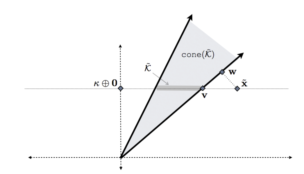
Here’s what the different elements in the image represent:
- $\tilde{K}$: This is the original convex set $K$, “lifted” into a higher dimension. It’s represented by the horizontal line segment.
- $\text{cone}(\tilde{K})$: This is the convex cone generated by $\tilde{K}$. It’s the shaded region.
- $\tilde{x}$: This is a point outside the lifted set, corresponding to a point $x$ outside the original set $K$.
- $v$: This is the projection of $\tilde{x}$ onto the lifted set $\tilde{K}$.
- $w$: This is the projection of $\tilde{x}$ onto the cone, $\text{cone}(\tilde{K})$.
- $\kappa \oplus 0$: This is the point $(\kappa, 0, \dots, 0)$ in the higher-dimensional space.
The key insight is that the distance from a point to the original set $K$ is related to the distance from the lifted point to the cone $\text{cone}(\tilde{K})$. Specifically: $$ \text{dist}(\tilde{x}, \text{cone}(\tilde{K})) \le \text{dist}(x, K) \le 2 \cdot \text{dist}(\tilde{x}, \text{cone}(\tilde{K})) $$ This means that if we can drive the distance to the cone to zero, we can also drive the distance to the original set to zero. With this trick in hand, the equivalence is established:
- From No-Regret to Approachability: A no-regret OLO algorithm can be used to solve an approachability problem by running it on the polar cone of the target set.
- From Approachability to No-Regret: An approachability algorithm can be used to solve an OLO problem by constructing a Blackwell instance where the set to be approached is the polar cone of the conic hull of the OLO decision set.
The geometric problem of steering an average payoff vector into a convex set, is fundamentally the same as, the algorithmic problem of minimizing regret in an online linear optimization setting.
So, given an approachable oracle algorithm $\mathcal{A}$, and a sequence of loss functions $f_1, \ldots, f_T$, the compact convex decision set $\mathcal{K} \subset \mathbb{R}^d$, one just needs to let the halfspace oracle $\mathcal{A}$ project the point, using the lifted payoff $u(\mathbf{x}, \mathbf{f}) : = \frac{\langle\mathbf{f}, \mathbf{x} \rangle}{\kappa} \oplus - \mathbf{f}$, to the cone, and use the iterative projection as your OLO algorithm. In the same spirit, given an OLO algorithm $\mathcal{L}$, one gets the iterative projection $x_t$ in the cone $\mathcal{K}$ by querying from the algorithm.
In short, Blackwell’s approchability determines how regret is vanishing. These two are sides of the same coin.